Short but not short enough
- Upasana Raval
- Sep 3, 2020
- 11 min read

If you have spent some mornings oversleeping in the arms of your warm blanket or if you have spent some evenings scrolling a mobile/TV screen infinitely, feeling guilty about skipping your exercise routine, you are not alone. A research study indicates that humans are innately lazy. The study finds the root cause of being lazy from the primitive days of humans and states “Conserving energy has been essential for humans' survival, as it allowed us to be more efficient in searching for food and shelter, competing for sexual partners, and avoiding predators.”
To circumvent any physical or mental exertion, our lazy brain finds out shortcuts for everything ranging from routine activities to long term milestones. Let’s explore this everyday problem of finding a way with minimal efforts, called a Shortest Path Problem, through the lens of math to sharpen our brain even further for its future endeavors.
A path to explore Shortest Path Problem
Formal definition
Brief history
Algorithms
Dijkstra’s algorithm
Example
Shortcomings
Complexity
Applications
Definition:
The formal definition of the Shortest Path Problem is rooted in Graph Theory – the study of graphs as related/connected objects. As per Wikipedia, Shortest Path Problem is “the problem of finding a path between two vertices (or nodes) in a graph such that the sum of the weights of its constituent edges is minimized.”
To understand this definition, it is important to know about graphs. A graph consists of vertices (nodes) that are connected by edges. These edges can be directed or undirected and weighted or unweighted. Edges in the directed graphs have specific directions to connect vertices while the undirected graphs have no specific direction. The weight on edges in the weighted graph represents any quantitative measure such as distance, time, cost, etc. that connects two vertices. Below is an example of a simple directed weighted graph. A, B, and C are the vertices representing cities. AB, AC, and BC are the edges representing paths connecting the cities. The numbers on the edges are the distance between the cities (weights). The direction of the edge, AB, suggests that there is a path to go from A to B but there is no path from B to A.

The Shortest Path Problem in this context is to find a path with minimum total weight between two nodes. For example, the shortest path between A to C is A – B – C with the minimum weight of 15. This problem is often called a single-pair shortest path problem.
There are three more variations of the Shortest Path Problem:
Single-source shortest path problem – find shortest path from a source vertex to all other vertices
Single-destination shortest path problem – find shortest path from all vertices to a single destination vertex
All-pairs shortest path problem – find shortest path between all pairs of vertices
History:
Early history of the Shortest Path Problem suggests that due to the glaringly elementary nature of the problem, it did not attract the mathematical research community until the mid-1950s. Interestingly, the need to solve the Shortest Path Problems programmatically came from various fields like information networks, economics of transportation, routing long distance telephone calls, etc. and several researchers developed the algorithms independently during the 1950s. Some of the popular algorithms are, Bellman-Ford algorithm (single-source SPP), Dijkstra's algorithm (single-source SPP), and A* search algorithm (single-pair SPP). The Shortest Path Problem can also be defined in terms of Linear Programming which is another exciting and vast field to immerse yourself into some other day.
For this article, I have decided to take you on a ride (not the shortest I am afraid) to learn about Dijkstra’s algorithm, for its simplicity, its applicability, and its cute little invention trivia.
Okay, so first trivia in Edsger Dijkstra’s words:
… One morning I was shopping in Amsterdam with my young fiancée, and, tired, we sat down on the cafe terrace to drink a cup of coffee. I was just thinking about whether I could do this, and I then designed the algorithm for the shortest path. As I said, it was a 20-minute invention …
And now the algorithm through an example:
It is a beautiful sunny morning in the upper east side of the New York City. More people are coming out to get away from their congested residences since the loosened shackles of covid-19 lockdown. For a change, I have put my Netflix = laziness to sleep and have decided to accompany the fresh air of Central Park while eating takeout food under the shade of a wise tree. Since time seems stagnant during the pandemic, my concern is not to reach the destination in the shortest amount of time but is to navigate through the stream of people walking towards their destination or sitting outdoors on the narrow streets of the neighborhood. My goal is to avoid as much crowd as possible on the way to pick up my lunch and to finally reach Central Park.
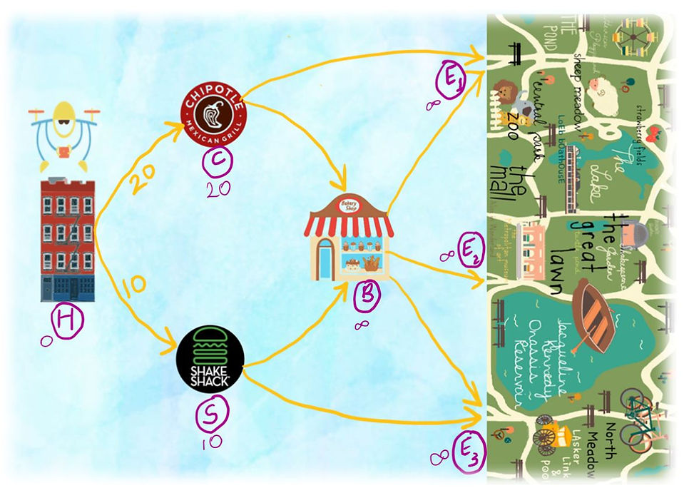
I have nothing to worry about. Skipper – my pet drone – is super charged to help me as usual. I have fed him a special morning snack – Dijkstra’s algorithm – along with the location of my preferred take out places. Below is the graph transformed by Skipper to represent my starting point (home - H), preferred take out places (C, S, and B), and final destination (Central Park – E1, E2, E3) as stops (vertices) and simplified paths (edges) leading to each stop. Skipper has this extraordinary capability of scanning and quantifying the crowd on any street into a score. Let’s call it a Crowd Score. Okay, so what does Skipper do? Essentially, Skipper starts from the start stop, scans neighboring stops, updates their Crowd Score, remembers the previous stop that keeps the current stop’s Crowd Score the lowest, and jumps to the next stop that has the lowest Crowd Score. This logic intuitively works as you imagine the shortest path between two vertices being made of smaller shortest paths between all the vertices on the way.

Let’s look at a bit formal logic, the pseudocode of Dijkstra’s algorithm, that I have fed to Skipper.
Skipper
Initially assigns Crowd Score of very high value (infinity) to all the stops since it is unknown in the beginning
Assumes Crowd Score of 0 for the Home stop to start with
Maintains the list of stops that are not yet visited, which will be all the stops in the beginning
Until all the stops are visited
Selects a stop a that is not yet visited and has minimum Crowd Score
Marks stop a as visited, meaning extracts stop a from the list of not visited stops
Scans all the stops b connected to stop a that belong to the list of not visited stops
Assigns stop b a Crowd Score of stop a + Crowd Score to reach to stop b from stop a, if the current Crowd Score of stop b is higher than the sum
Worry not if some of these words fell off your attention. Skipper will be reporting live from the sky to illustrate the implementation of this logic.
Here we go, to find the best path to reach Central Park with minimum crowd exposure = Crowd Score.
Skipper is at starting point H and is in the initialization mode

Below is the summary report that Skipper sends from each stop. The report is now in the initialization stage of the algorithm. Our starting stop H is initialized with zero Crowd Score and the rest of the stops are initialized with infinity Crowd Score since we do not yet know the value for them. As H has the minimum Crowd Score of all, it has been extracted from the not visited list. The column previous stop is to keep track of the stop Skipper traversed before the stop in focus. This tracking will help to trace the best path once all the stops are visited and the algorithm is over. The list of visited and not visited stops is maintained in the top most area with gray coloured text. This list helps pick the next stop to visit.

As per the pseudocode, the next step is to scan the neighboring stops, C and S, connected to the current stop H. Skipper scanned and reported the Crowd Score to reach stops C and S from stop H as following.
Now, the Crowd Scores for C and S are updated in the report as per the below logic.
Crowd Score of C = min (Crowd Score of C, Crowd Score of H + Crowd Score of H to C)
= min (infinity, 0 + 20)
= 20
Crowd Score of S = min (Crowd Score of S, Crowd Score of H + Crowd Score of H to S)
= min (infinity, 0 + 10)
= 10
H is declared as a previous stop for C and S for their adjacency to stop H. This gets updated in the previous stops column. Skipper has already hinted to go to the next stop, S, because it has the lowest Crowd Score out of all the not visited stops.

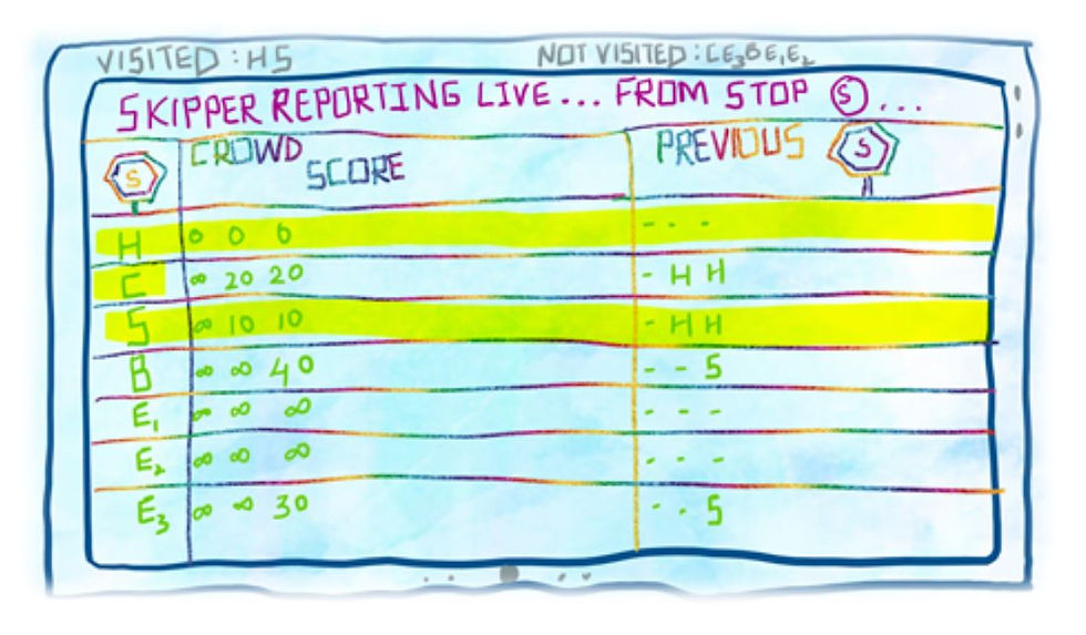
2. Skipper is at stop S
Skipper has scanned the neighboring stops, B and E3 from stop S and has reported their respective Crowd Scores from S.
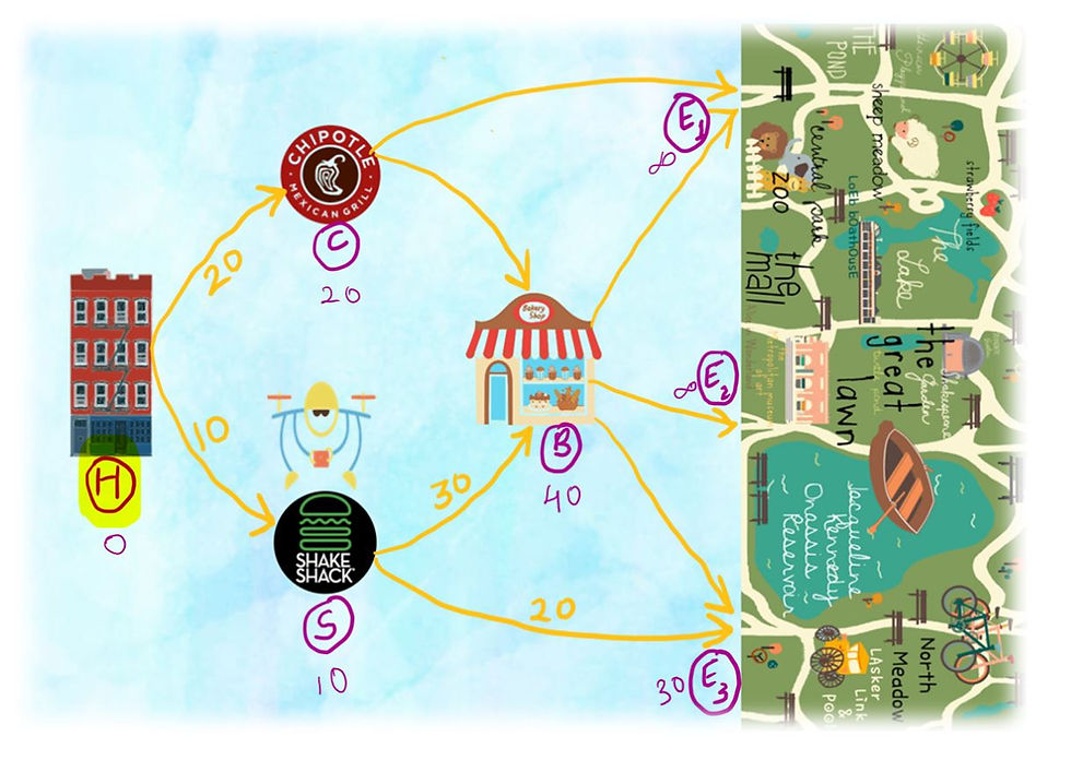
Crowd Score of B = min (Crowd Score of B, Crowd Score of S + Crowd Score of S to B)
= min (infinity, 10 + 30)
= 40
Crowd Score of E3 = min (Crowd Score of E3, Crowd Score of S + Crowd Score of S to E3)
= min (infinity, 10 + 20)
= 30
The summary report is updated with the Crowd Score for B and E3. Now, Skipper is hinting to go to the next stop, C, because it has the lowest Crowd Score out of all the not visited stops.
3. Skipper is at stop C
Neighboring stops B and E1 have been scanned to find out Crowd Score from C. It is to remind that stop B is scanned second time since it is still on the list of not visited stops. Let’s see if B’s score is improved from C compared to its current score from S.

Crowd Score of B = min (Crowd Score of B, Crowd Score of C + Crowd Score of C to B)
= min (40, 20 + 10)
= 30
Crowd Score of E1 = min (Crowd Score of E1, Crowd Score of C + Crowd Score of C to E1)
= min (infinity, 20 + 30)
= 50
As per the calculation, B’s score is reduced to 30 from 40 and the previous stop in the report has been updated to be C instead of S.
The summary report now shows the updated scores for B and E1. There is a tie for Skipper to break since the Crowd Scores of stop B and E3 are the same. Skipper is breaking the tie with alphabetical order and is off to the next stop B. Hurray!! We are almost there!

4. Skipper is at stop B
Crowd Scores from stop B to all the neighboring stops E1, E2, and E3 are scanned. Let’s see how the Crowd Scores of these stops are updated in the report.

Crowd Score of E1 = min (Crowd Score of E1, Crowd Score of B + Crowd Score of B to E1)
= min (50, 30 + 10)
= 40
Crowd Score of E2 = min (Crowd Score of E2, Crowd Score of B + Crowd Score of B to E2)
= min (infinity, 30 + 30)
= 60
Crowd Score of E3 = min (Crowd Score of E3, Crowd Score of B + Crowd Score of B to E3)
= min (30, 30 + 10)
= 30
As per the calculations, the E1 now has better Crowd Score than before from stop B.
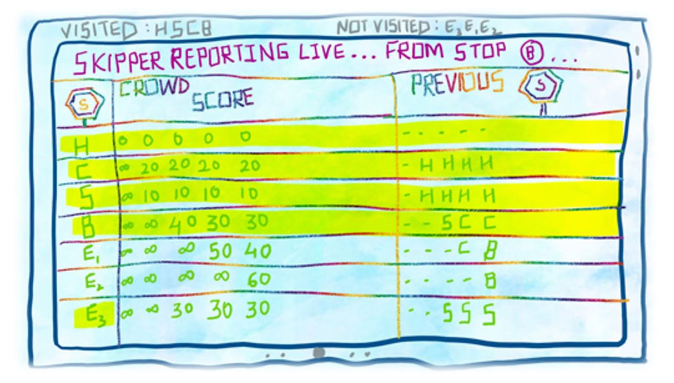
We now have non-infinity scores for all the stops. However, we are yet to traverse to three more nodes E1, E2, and E3. At this point, it is quite trivial to claim that Crowd Scores of all the stops and their respective previous stops would not change since the remaining three nodes are the end nodes, meaning they are not further connected to any other nodes in the graph.
Skipper will do his due diligence to traverse to the remaining nodes anyway. Mental note: the order of travel to these nodes will be E3 -> E1 -> E2 as per the rule of traveling and extracting minimum Crowd Score stop. Here is how it looks in fast-forward.
5. Skipper is at stop E3

6. Skipper is at stop E1

7. Skipper is at stop E2

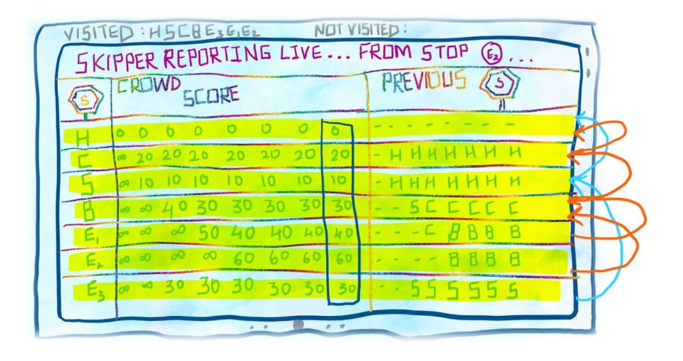
The “shortest path” (minimum Crowd Score path) from H to every other stop can be derived by tracing previous stops from the final report. Crowd Score for each path is the Crowd Score from last iteration (last column)
Below are the final paths and associated Crowd Scores.

Good job Skipper! Show me the snippet of your travel.
Tell me, am I getting any cake today on the way to Central Park? And the answer is no :/ because the path entering Central Park with the least Crowd Score is H -> S -> E3, meaning Home -> Shake Shack -> Central Park Entrance 3. Sob sob…. Well, I can still get a Chocolate shake from Shake Shack anyway!
Shortcoming:
One drawback of using Dijkstra’s algorithm is that it fails to find the shortest path when any edge has a negative weight. Why? The algorithm never re-visits and updates the value of any vertex that has already been visited as the vertex is visited only when it has the minimal value to begin with. This logic works when you have only positive weights, addition of positive weights can never decrease in value. However, when you have negative weights, addition of positive weights can decrease. Therefore, the algorithm cannot guarantee to find the shortest path in that case. If you want to take a little fun detour, try changing the Crowd Score of the path connecting S and E3 to 5 and the path connecting B and E3 to -30 to see how the algorithm fails to determine the path with minimum Crowd Score from H to E3. One way to tackle this shortcoming is to add positive weight to all the edges equivalent of the most negative weight on a given edge. Another solution could be to use the Bellman-Ford algorithm which can tackle negative weights. The Shortest Path Problem becomes intractable when there is a negative cycle in the graph like the one shown below. Here a cycle is formed from A – B – C and has a total weight of -5 for the same.

Another basic assumption which may not hold true in real life is that the value between two vertices remains stationary, for example, it is possible that the time to travel between two locations can vary based on the time of the day, day of the week, weather, etc. In that case, the shortest path found might not be truly shortest.
Complexity of Dijkstra’s algorithm:
Where there is an algorithm, there is a complexity! Complexity (run time) of an algorithm in simple terms is determined by the number of steps performed during its implementation. This can become a very specific and tedious calculation for each input graph. Therefore, the complexity is always approximated based on the size of the input data.
For the classic implementation of Dijkstra’s algorithm that we covered, the complexity is of the order of V2 where V is the number of vertices in the graph. This is because of the two main tasks performed in the algorithm.
Find the vertex with minimum value (Crowd Score in the example) – this can take V steps at the most
Update value of the neighboring vertices – this can also take V steps at the most
There are modern implementations of Dijkstra’s algorithm that leverage efficient data structures resulting in better run times.
Applications of Shortest Path:
There are many applications of the Shortest Path in real life. The most popular theme to use shortest path algorithms is for routing between locations/devices. It can be routing of people, trucks, flights, emergency response vehicles, robots, telecommunication messages, network protocols, etc. Shortest path algorithms can also be leveraged to find out betweenness or degree of separation between two people in a social network. Another interesting application is to design process maps of emergency response systems in order to reach the end goal in the most efficient way. A fun application for the shortest paths is to win the games like Snakes and Ladder in the minimum number of dice rolling when the dice gives the number of your dreams ;-) The most fascinating application to me is to find arbitrage opportunities in currency exchange. What order should I follow to exchange currency to make the maximum profit out of it?
And here our ride ends! I hope this article has ignited your curiosity enough to continue exploring many more interesting and relatable math problems. Who knows, someone could be writing about how you invented your algorithm while eating lunch under the shade of a wise tree in Central Park in 2030!
Acknowledgements:
I would like to thank Mainak Mustafi, Prachi Pande, and Girish Krishnan for reviewing this article. A special thanks to Charu Mehta for being amazingly inspiring!
References:
Research paper on human tendency to avert exertions- https://www.sciencedirect.com/science/article/abs/pii/S0028393218303981?via%3Dihub
Nice slides explaining Dijkstra’s algorithm, implementations, complexity, proof, applications- https://www.cs.princeton.edu/~rs/AlgsDS07/15ShortestPaths.pdf
Interactive explanation of Dijkstra’s algorithm- https://www-m9.ma.tum.de/graph-algorithms/spp-dijkstra/index_en.html
Dijkstra trivia - https://www.cs.cornell.edu/courses/JavaAndDS/shortestPath/01shortestPathHistory.pdf
Image Credits:
Central park illustration: https://www.theydrawandtravel.com/illustrations/5705-central-park-in-new-york-new-york
Home building illustration: https://wdrfree.com/stock-vector/brownstone


So me being lazy is just evolution, that is good to know!!! 😬😬😬😬