The cosmic distance ladder and the expanding universe
- Amol Patwardhan
- Jul 17, 2020
- 15 min read
Celestial bodies have been a source of fascination to humans since time immemorial. For millennia, we have observed and documented their motions through the sky, and tried to understand it all in terms of a unified framework of the underlying physical laws, such as the law of gravitation. Central to this enterprise has been an effort to accurately measure or infer just how far away these objects are from us.
The known range of distances in astronomy is enormous, spanning nearly 18 orders of magnitude. At one end, sits the Earth-Moon distance of about 384,400 kilometres; at the other end are the most distant galaxies observed till date, more than 13 billion light years away, or roughly 120,000,000,000,000,000,000,000 km (120 billion trillion km)!
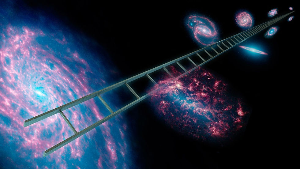
Naturally, it would be fair to expect that no single measurement technique can suffice on its own in the determination of astronomical distances over such a vast range of scales. This necessitates the development of a “cosmic distance ladder”, wherein a variety of techniques are used in a hierarchical fashion, starting from the nearest objects and culminating at the most distant ones. At each step of the ladder, techniques whose reliability is established up to a certain distance are used to calibrate* other techniques which have the capacity to measure out to farther distances. This requires that, at each step, there be an overlap— that is, there should exist a range of distances where two techniques can be simultaneously utilized, in order for one of them to be calibrated against the other.
* - This process of ‘calibration’ can be explained using a simple analogy. Imagine having two rulers, a short one where the markings on the rulers have a known unit, such as centimetres or inches, and a longer one where the unit on the markings is unknown. In this scenario, before the longer ruler can be used for any meaningful measurement, the scaling between the two units needs to be established by placing the two rulers side-by-side.
It has been known, for almost a century, that our universe is undergoing expansion. That is to say, on average, galaxies in the universe appear to be moving further apart from one another. One of the most important applications of the cosmic distance ladder has been to measure the expansion rate of the universe. Measuring the expansion rate is a crucial step towards understanding the composition of the universe, as well as potentially its origin.
In the first part of this article, we give some examples of distance determination techniques at various rungs of the cosmic distance ladder, illustrating how the process of calibration works from one rung to the next. In the second part, we discuss the use of these techniques in the determination of the ‘Hubble constant’, which is a measure of the expansion rate of the universe. Lastly, we touch upon a current hot topic of intrigue in cosmology— namely, the ‘Hubble tension’, i.e., a disagreement between the values of the Hubble constant as inferred by different methods.
Part 1: The cosmic distance ladder
§ 1.1. Direct distance measurements
At the lowest rung of the cosmic distance ladder are what we call "direct" or "fundamental" distance measurements, wherein no assumption is needed about the physical nature of the object, such as its size or brightness. To begin with, distances to nearby objects in the solar system can be measured by reflecting electromagnetic radiation* off them. Since the speed of electromagnetic radiation is a known fundamental constant, measuring the round-trip duration between emission and detection allows for a determination of the surface-to-surface distance. An example of this is the Lunar Laser Ranging Experiment— where laser pulses from earth-based observatories are aimed at retro-reflectors that were installed on the moon during the Apollo missions. By precisely measuring the orbit of the moon, this technique can also be used to test different theories of gravity— including Einstein’s general theory of relativity [1].
* - As a reminder, electromagnetic radiation encompasses, from low to high frequencies, the following types of radiation: radio waves, microwaves, infrared light, visible light, ultraviolet light, X-rays, and gamma rays). The speed of any electromagnetic wave in vacuum is the same as the speed of light— 299,792,458 meters per second.
Another example is Radar astronomy, where microwaves are reflected off target objects within the solar system. This technique has the additional benefit of also being able to gather information about the shapes, sizes, and surface properties of the target objects. Within the solar system, the interplanetary distances keep on changing as the planets move along the orbits, so the distances by themselves carry no particular meaning. However, a precise measurement of interplanetary distances as a function of time allows us to determine the relevant parameters of the planetary orbits, such as the orbital radius and degree of ellipticity. In particular, radar measurements of Venus have been used for obtaining a high-precision measurement of the Earth’s own orbital radius [2].
Kepler’s third law states that the cube of the orbital radius (or to be precise, the semi-major axis for an elliptical orbit) is proportional to the square of the orbital period. The proportionality constant depends on the mass of the central object (in this case, the Sun). A direct measurement of the orbital radii and periods of nearby planets enables us to determine this proportionality constant, which can then in turn be used to infer the orbital radii of the remaining planets by measuring their periods.
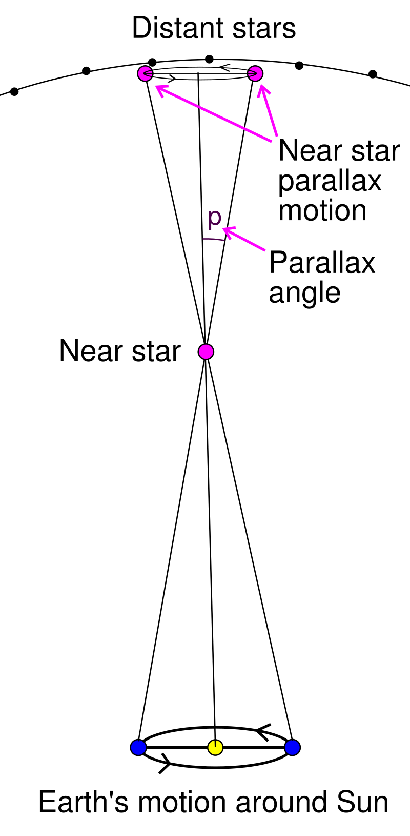
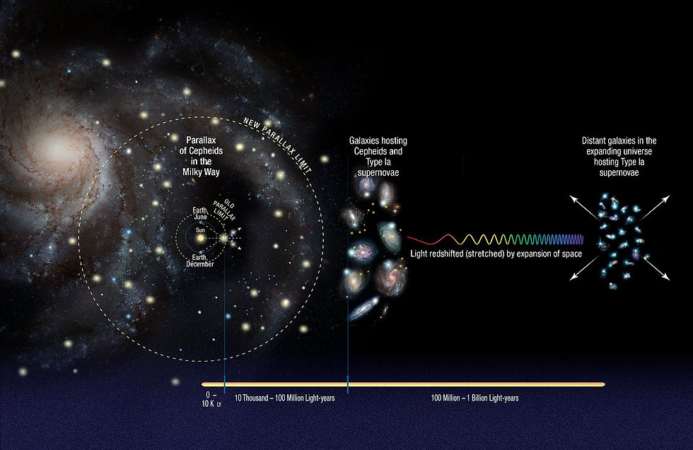
Direct distance measurements using electromagnetic wave reflection are not useful outside the solar system, because the strength of the electromagnetic signal reflected and received back at the earth diminishes with the square of the distance to the target, and therefore becomes unmeasurable at a certain point. The next rung of the cosmic distance ladder instead makes use of the simple concept of parallax. Parallax is the word used to describe the apparent change in the position of an object relative to a distant background, when viewed from different locations. In the astrophysical context, this effect results in the shifting of the apparent angular positions of nearby stars, relative to the background of more distant stars, as the Earth moves along its orbit around the Sun. In fact, trigonometric parallax is used to define a new distance unit— the parsec— used commonly in astronomy. One parsec is defined as the distance to an object whose parallax angle (see adjoining image) as calculated with respect to the Earth’s orbit is 1 arc second. One parsec is approximately 3.26 light years. Here, it is important to note that the process of determining distances through parallax thus relies on a robust measurement of the earth’s orbit around the sun, which can be accomplished at the lowest rung of the distance ladder through the direct electromagnetic-wave-based measurement methods described above.
In practice, the angular shifts in the apparent positions of objects outside the solar system as a result of parallax are too tiny to be discernible to the naked eye— even Alpha Centauri, the nearest star to our solar system, has a parallax angle of less than one arc-second (or 1/3600th of a degree). But with state-of-the-art astronomical instruments, such as the “Wide Field Camera 3” on the Hubble Space Telescope (abbreviated as HST— the word ‘Hubble’ in the text henceforth refers to the scientist and not to the telescope) with a 20-40 micro-arc-second angular resolution, the method of parallax has the potential to calculate distances of objects up to 5000 parsecs from the sun. For comparison, the diameter of the Milky Way galactic disk is about 30,000 parsecs, so even with our best telescopes, the furthest reach of this technique still only spans a nearby region within our own galaxy.
§ 1.2. Indirect distance measurements
Technically speaking, the method of parallax can be considered a direct or fundamental distance measurement, since no assumption is made regarding the intrinsic properties of the object in question. However, in order to extend the reach of the cosmic distance ladder to the far end of the galaxy and beyond, one increasingly starts to depend on the knowledge of the object’s intrinsic properties, in particular, its luminosity (i.e., energy output per unit time). Such types of objects— called “Standard Candles”— have a luminosity that is either known (based on identifying what type of object it is), or can be inferred based on its other observable properties. Knowing the luminosity of an object, and by measuring its apparent brightness as observed from earth (quantified in terms of the measured light flux, i.e., energy received per unit area per unit time), the distance to the object can be calculated using the fact that the apparent brightness scales as the inverse square of the distance. Here, we shall present two examples of such Standard Candles.
The first example is a type of star known as a “Cepheid variable”. Variable stars, in general, are stars whose apparent brightness changes periodically with time. In some cases the change is because of external factors such as the star being eclipsed by a companion star*
or a planet. However, in other cases, the change in brightness is intrinsic. These changes may be caused, for instance, by pulsations of the star, i.e., periodic expansion and contraction as the star attempts to reach a state of equilibrium between pressure and gravity. Cepheid variables are a particular class of pulsating star which can be identified by their distinctive sawtooth shaped lightcurves (i.e., curves showing the variation of luminosity with time).
* - A large percentage of stars, perhaps even a majority, are found in binary systems, i.e., as a pair orbiting around their common center of gravity.
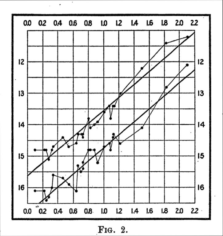
In 1908, Henrietta Swan Leavitt, through her study of variable stars in the Large and Small Magellanic Clouds (satellite galaxies of the Milky Way), discovered that there exists a definite relationship between the pulsation period and the apparent brightness of these Cepheid variable stars— the brighter of these stars had longer pulsation periods. In a subsequent study from 1912 [3], she analyzed a sample of 25 Cepheid variables from the Small Magellanic Cloud, and demonstrated an approximate linear relationship between the logarithm of the apparent brightness, and the logarithm of the pulsation period. The figure on the left, reproduced from that paper, shows this relationship between apparent brightness (y-axis) vs pulsation period (x-axis). Both axes are on a logarithmic scale, and the points along the upper and lower curves correspond to the maximum and minimum brightness of each star.
Leavitt reasoned that since all the 25 stars here resided within the Small Magellanic Cloud, they were all at approximately the same distance from us, and therefore the apparent brightness of each star could be used as a proxy for its intrinsic luminosity, up to some unknown constant multiplicative factor. Therefore, a relationship between pulsation period and apparent brightness could be interpreted as a relationship between pulsation period and luminosity, with the unknown multiplicative factor requiring calibration via measurements of stars with known distances. Over the years, parallax measurements of Cepheid variable stars within our own galaxy have enabled this period-luminosity relation to become increasingly better calibrated. This is another example of a lower rung of the cosmic distance ladder being used to calibrate an upper rung.
One of the first known applications of the period-luminosity relation was carried out by Edwin Hubble in 1924, who used it to calculate the distances of Cepheid variable stars in what was then known as the Andromeda Nebula. His work led him to conclude that these stars were too far away to be a part of our own galaxy, and therefore, the Andromeda “nebula”, in fact, had to be a galaxy of its own. His work was subsequently published in 1929 [4].
Cepheid variable stars can be quite luminous by stellar standards (up to 100,000 times more luminous than the Sun). Nevertheless, they have a limited reach in terms of being distance indicators. They have their utility within the Milky way, in neighboring galaxies such as Andromeda, about 2.5 million light years away, and in nearby clusters of galaxies such as the Virgo cluster, about 55 million light years away. However, at farther distances, it becomes increasingly difficult to optically resolve individual stars, and therefore other standard candles become necessary.
Enter Type Ia supernovae (read: type one-a). Supernovae are explosions of stars in the final stages of their life cycle. Often, these explosions can be so bright that they even briefly outshine their entire host galaxy, and can therefore be seen from very far away. Type Ia supernovae are a particular class of stellar explosions which can arise in binary star systems where one of the stars is a white dwarf. White dwarfs are formed when ordinary stars like the sun burn out their nuclear fuel and undergo contraction to form a compact but extremely dense object (about a million times denser than water). In some cases, white dwarfs that are part of a binary star system can accrete matter from their companion star, and undergo a spectacular thermonuclear explosion once they reach a critical mass threshold. Because all Type Ia explosions occur at about the same critical mass (roughly 1.4 times the mass of the Sun), the variation in their luminosity is fairly small, enabling their use as standard candles.
The calibration of the luminosity scale of Type Ia supernovae can be performed using Cepheid variable stars. That is, Cepheid variables can be used to calculate the distance to nearby host galaxies containing Type Ia supernovae, and then the luminosity can be calculated using this distance and the observed apparent brightness. Once calibrated, the Type Ia supernovae can then in turn be used as standard candles in galaxies that are much further away, on account of them being so exceedingly bright.
Of course, it goes without saying that there exist several other methods to determine cosmic distances (praise be to Wikipedia). For example, the recent instances of gravitational wave detection from the inspirals and mergers of binary black holes and binary neutron star systems, has led to the use of these events as “Standard sirens”. Based on the observed waveform of the detected gravitational wave signal, the total power emitted in gravitational waves at the source can be computed. This can then be compared with the recorded signal strength to get an estimate of the distance to the source.
Each of these methods, including the ones described here, is laced with various caveats and pitfalls. It is of course, entirely possible that the so-called Standard candles are not as standard as hoped, and could exhibit variations depending on factors such as composition and environment. For instance, it was discovered by Walter Baade in 1950 that the nearby Cepheid variables used for calibration had a higher metallicity compared to the Cepheids used to measure the distances to nearby galaxies, and therefore they had to be calibrated differently. This led to the doubling of the distances to nearby galaxies that were measured by Hubble, and a revision of his estimate for the age of the universe. Other potential issues with use of standard candles may include, for example: 1. mis-identifying a source as belonging to a standard candle class when it actually does not; or 2. failure to properly account for extinction of light caused by interstellar or intergalactic gas and dust. Moreover, as each rung of the distance ladder is calibrated against the previous one, this leads to a propagation of errors across each step.
Despite these obstacles, the use of the cosmic distance ladder has enabled a vast amount of progress in our understanding of the structure, evolution, and composition of the universe. Few examples illustrate this better than the story of the expanding universe.
Part 2: The expanding universe

In 1915, Vesto Slipher observed that the light coming from most galaxies appeared to be redshifted [5]. Redshifting of light is caused by the Doppler effect, whereby the light emanating from a receding object is perceived to have a lower frequency (or a longer wavelength), and therefore appears redder (the same phenomenon— lowering of the measured frequency from a receding source— is also observed in sound waves). The amount of redshift is directly proportional to the velocity of the receding object, hereafter called the “recession velocity”. Slipher was thus able to conclude that most galaxies appeared to be receding from the Milky way, and he calculated their recession velocities.
Around this time, Albert Einstein developed his theory of general relativity, and one of the predictions of this theory was that the universe could not be static*. In 1922 and 1927, respectively, Alexander Friedmann and Georges Lemaître independently derived the equations for the expanding universe, starting from Einstein’s field equations of general relativity. In 1929, Edwin Hubble used Cepheid variable stars to measure the distances to several galaxies, and combined it with Slipher’s and Milton Humason’s measurements of recession velocities to discover that, on average, the recession velocities were proportional to the distances to the galaxies [6].
* - Einstein did not like the concept of a non-static universe, and attempted to fix his theory by introducing an additional parameter, called the ‘Cosmological constant’— this led to a universe that was static, but nevertheless unstable. Eventually, he abandoned the cosmological constant idea, calling it his “biggest blunder”, once Hubble established in 1929 that the universe was indeed expanding, and therefore not static. Interestingly enough, the cosmological constant idea got revived much later for a different purpose, once it was discovered (in the 1990s) that the expansion of the universe was accelerating. It now constitutes the simplest theoretical explanation of the “Dark Energy” hypothesis.
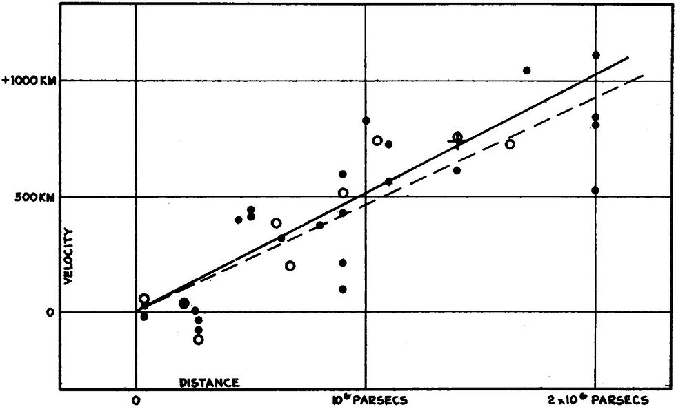
The figure on the left, reproduced from Hubble's 1929 paper, demonstrates this relationship between recession velocity (in km/s) and distance (in parsecs). The black disks and solid line correspond to the data set where each galaxy is treated separately, whereas the white disks and dashed line correspond to the data set where the 24 galaxies are divided into 9 groups based on proximity. The cross represents the mean distance and velocity of 22 galaxies whose distances could not be measured individually.
The proportionality constant between the two quantities has since come to be known as the “Hubble constant”, even though the value inferred by Hubble was almost an order of magnitude higher compared to the much more accurate modern-day measurements. This relationship between recession velocity and distance was also noted by Lemaître in his 1927 paper [7], but since it was published in a little known Belgian journal, he was not as widely credited for it*. Hubble’s use of Cepheid variables meant that he was looking at relatively nearby galaxies, and as a result there was a considerable amount of spread in the data, caused by local gravitational effects.
* - In 1931, an English translation of Lemaitre's work was published in the Monthly Notices of the Royal Astronomical Society, however, some of the key points, including Lemaitre's derivation of Hubble’s law and his estimates of the proportionality constant, were left out. It has emerged that the omission was carried out at Lemaitre's own behest, since he considered those results as provisional and not of great interest [8].
In modern times, the measurement of the Hubble constant, more appropriately known as the “Hubble parameter” (since the ratio of recession velocity to distance is not constant in time— it decreases over time as the universe expands), has become much more sophisticated. Notably, using observations of Type Ia supernovae, it has become possible to measure the change in the Hubble parameter with distance (or equivalently, with cosmic time— remember that observing far out in space is the same as observing far back in time). This has been used to demonstrate that the expansion of the universe is actually accelerating [9,10]. This discovery was recognized with the 2011 Nobel prize in physics.
Moreover, the value of the Hubble parameter can now be inferred using nearly a dozen different methods [11,12]. In the process, some tensions have been revealed between the inferred best-fit values of the Hubble parameter as determined by the different techniques. In particular, the best-fit value of the Hubble parameter inferred from observations of Cepheid-calibrated Type Ia supernovae is in significant tension (4.4 standard deviations) with the value inferred from measurements of the Cosmic Microwave Background (CMB) radiation by the Planck satellite. The CMB is the leftover relic electromagnetic radiation from the Big bang, that decoupled from the hot, primordial plasma in the early universe when it cooled enough to allow electrons and nuclei to combine into atoms. Therefore, a measurement of this radiation essentially amounts to an observation of this decoupling epoch, which occurred when the universe was only about 375,000 years old (the current age of the universe is known to be about 13.8 billion years). The value of the Hubble parameter, as well as that of a number of other cosmological parameters, can be inferred through a statistical analysis of the anisotropies (i.e., directional dependence) in the temperature and polarization of the CMB radiation.
However, it must be noted that the values of present-day cosmological parameters as inferred from the CMB data constitute an indirect measurement. The CMB data reflects the state of the universe at a much earlier time, and in order to interpret what that data represents in the present-day universe, one must assume a theoretical model that describes how the universe evolved during the intervening period. As a result, while it is still possible that the tension between the two independent methods could be arising as a result of unforeseen systematic errors in one or both of these methods, it has nevertheless called into question whether the standard ΛCDM (read: Lambda-CDM) cosmological model of the universe, consisting of a dark energy component that is a cosmological constant, and a dark matter component that is cold and collisionless, requires considerable modifications.
Whatever it may be, there is certainly no doubt that exciting times lie ahead in this field!
References:
Cited in-text:
"APOLLO": https://tmurphy.physics.ucsd.edu/apollo/apollo.html
"To See the Unseen, chapter two: Fickle Venus": https://history.nasa.gov/SP-4218/ch2.htm
"Periods of 25 Variable Stars in the Small Magellanic Cloud", Leavitt, Henrietta S.; Pickering, Edward C., Harvard College Observatory Circular, vol. 173, pp.1-3, March 1912: https://ui.adsabs.harvard.edu/abs/1912HarCi.173....1L/abstract
"A spiral nebula as a stellar system, Messier 31", Hubble, E. P., Astrophysical Journal, 69, 103-158, March 1929: https://ui.adsabs.harvard.edu/abs/1929ApJ....69..103H/abstract
"Spectrographic Observations of Nebulae", Slipher, V. M., Popular Astronomy, Vol. 23, p. 21-24, January 1915: https://www.roe.ac.uk/~jap/slipher/slipher_1915.pdf
"A relation between distance and radial velocity among extra-galactic nebulae", Hubble, Edwin, Proceedings of the National Academy of Sciences of the United States of America, Volume 15, Issue 3, pp. 168-173, March 1929: https://www.pnas.org/content/pnas/15/3/168.full.pdf
"Un Univers homogène de masse constante et de rayon croissant rendant compte de la vitesse radiale des nébuleuses extra-galactiques", Lemaître, G., Annales de la Société Scientifique de Bruxelles, A47, p. 49-59, 1927: https://ui.adsabs.harvard.edu/abs/1927ASSB...47...49L/abstract; English translation: "Expansion of the universe, A homogeneous universe of constant mass and increasing radius accounting for the radial velocity of extra-galactic nebulae", Lemaître, G., Monthly Notices of the Royal Astronomical Society, Vol. 91, p.483-490, March 1931: https://ui.adsabs.harvard.edu/abs/1931MNRAS..91..483L/abstract
"Lost in translation: Mystery of the missing text solved", Livio, Mario, Nature, Volume 479, Issue 7372, pp. 171-173, November 2011: https://www.nature.com/articles/479171a
"Measurements of Ω and Λ from 42 High-Redshift Supernovae", Perlmutter, S. et al., The Astrophysical Journal, Volume 517, Issue 2, pp. 565-586, June 1999: https://iopscience.iop.org/article/10.1086/307221
"Observational Evidence from Supernovae for an Accelerating Universe and a Cosmological Constant", Riess, Adam G. et al., The Astronomical Journal, Volume 116, Issue 3, pp. 1009-1038, September 1998: https://iopscience.iop.org/article/10.1086/300499
"Investigating the Hubble Constant Tension -- Two Numbers in the Standard Cosmological Model", Lin, Weikang; Mack, Katherine J.; Hou, Liqiang: https://arxiv.org/abs/1910.02978
"Hubble Constant, H0": https://lambda.gsfc.nasa.gov/education/graphic_history/hubb_const.cfm
Not cited in-text:
Comments